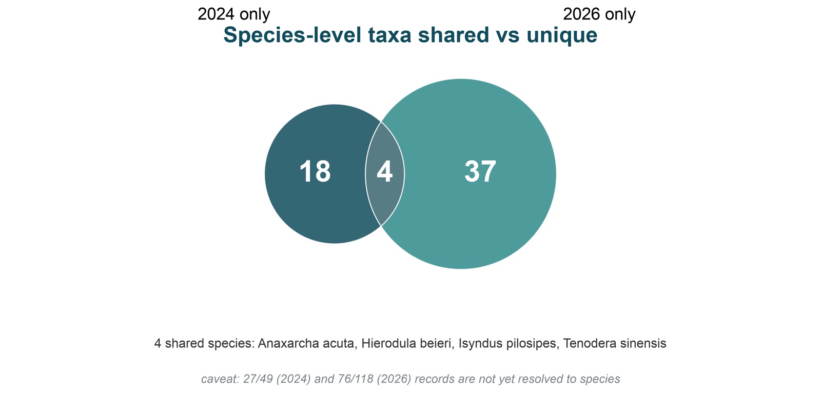
Species composition shifts with season: nocturnal insect surveys in Medog, SE Tibet

Two short expeditions to Medog County (SE Tibet) were compared: 6–9 August 2024 (4 field days) and 26 June – 2 July 2026 (7 field days), both using nocturnal searching and light trapping. Records rose from 49 to 118 — a 2.4-fold difference that is explained by effort, not by a richer fauna: the per-day discovery rate barely moved (5.5 vs 5.9 species/day). Species composition was another matter. Only 4 of 59 species-level taxa were recorded on both expeditions, so turnover between early and late summer in this valley is high.

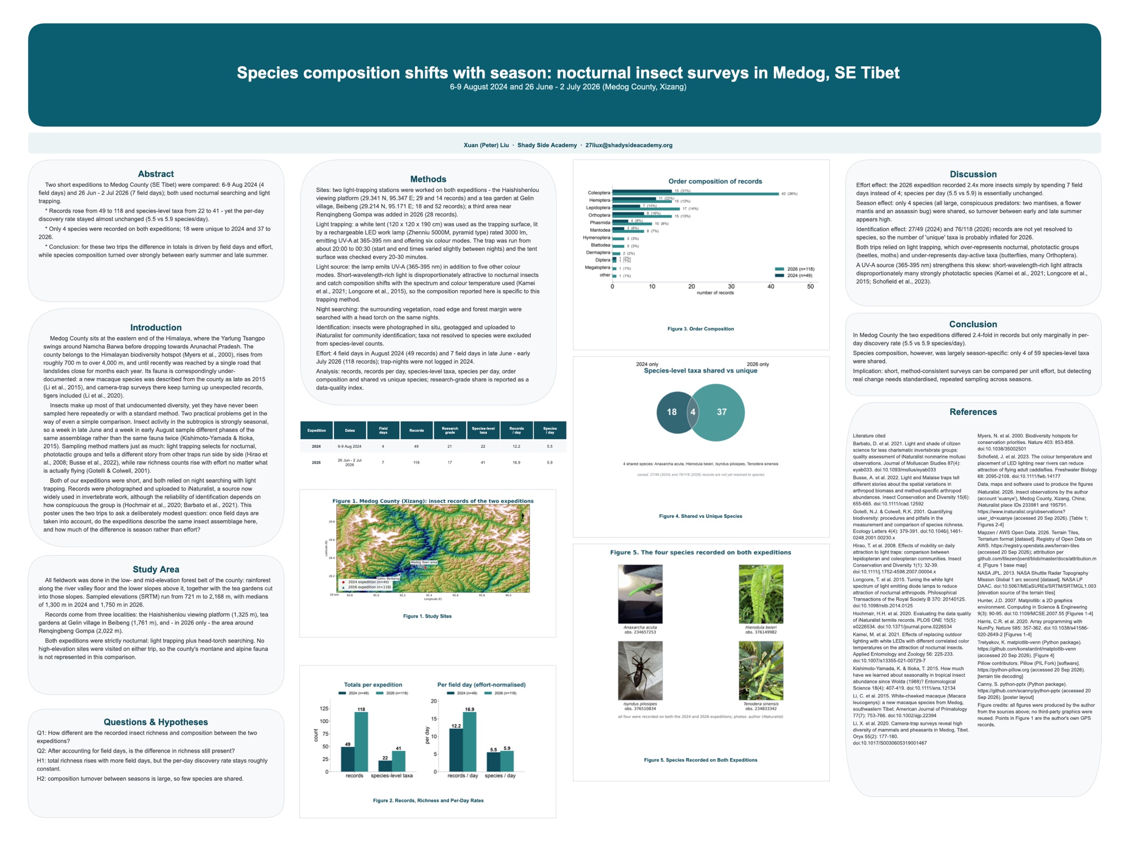
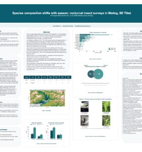
Species composition shifts with season: nocturnal insect surveys in Medog, SE Tibet. Research poster, 48 × 36 in. Xuan (Peter) Liu, Shady Side Academy. Click to open full size.

Abstract

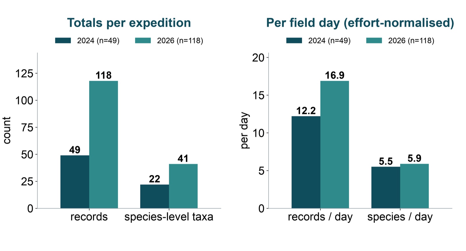
Records rose from 49 to 118 and species-level taxa from 22 to 41 — yet the per-day discovery rate stayed almost unchanged (5.5 vs 5.9 species/day).
Only 4 species were recorded on both expeditions; 18 were unique to 2024 and 37 to 2026.
Conclusion: the difference in totals is driven by field days and effort, while species composition turned over strongly between early summer and late summer.

Introduction

Medog County sits at the eastern end of the Himalaya, where the Yarlung Tsangpo swings around Namcha Barwa before dropping towards Arunachal Pradesh. It belongs to the Himalayan biodiversity hotspot (Myers et al., 2000), rises from roughly 700 m to over 4,000 m, and until recently was reached by a single road that landslides close for months each year. Its fauna is correspondingly under-documented: a new macaque species was described from the county as late as 2015 (Li et al., 2015), and camera-trap surveys there keep turning up unexpected records, tigers included (Li et al., 2020).

Insects make up most of that undocumented diversity, yet they have never been sampled here repeatedly or with a standard method. Two practical problems get in the way of even a simple comparison. Insect activity in the subtropics is strongly seasonal, so a week in late June and a week in early August sample different phases of the same assemblage rather than the same fauna twice (Kishimoto-Yamada & Itioka, 2015). Sampling method matters just as much: light trapping selects for nocturnal, phototactic groups and tells a different story from other traps run side by side (Hirao et al., 2008; Busse et al., 2022), while raw richness counts rise with effort no matter what is actually flying (Gotelli & Colwell, 2001).

Both expeditions were short, and both relied on night searching with light trapping. Records were photographed and uploaded to iNaturalist. This study uses the two trips to ask a deliberately modest question: once field days are taken into account, do the expeditions describe the same insect assemblage here, and how much of the difference is season rather than effort?

Study area

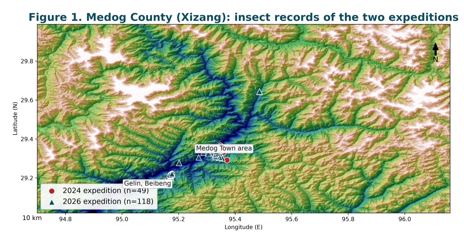
All fieldwork was done in the low- and mid-elevation forest belt of the county: rainforest along the valley floor and the lower slopes above it, together with the tea gardens cut into those slopes. Sampled elevations (SRTM) run from 721 m to 2,168 m, with medians of 1,300 m in 2024 and 1,750 m in 2026.

Records come from three localities: the Haishishenlou viewing platform (1,325 m), tea gardens at Gelin village in Beibeng (1,761 m), and — in 2026 only — the area around Renqingbeng Gompa (2,022 m). Both expeditions were strictly nocturnal. No high-elevation sites were visited on either trip, so the county’s montane and alpine fauna is not represented in this comparison.

Questions and hypotheses

Q1: How different are the recorded insect richness and composition between the two expeditions?
Q2: After accounting for field days, is the difference in richness still present?
H1: total richness rises with more field days, but the per-day discovery rate stays roughly constant.
H2: composition turnover between seasons is large, so few species are shared.

Methods

Sites. Two light-trapping stations were worked on both expeditions — the Haishishenlou viewing platform (29.341 N, 95.347 E; 29 and 14 records) and a tea garden at Gelin village, Beibeng (29.214 N, 95.171 E; 18 and 52 records); a third area near Renqingbeng Gompa was added in 2026 (28 records).
Light trapping. A white tent (120 × 120 × 190 cm) was used as the trapping surface, lit by a rechargeable LED work lamp rated 3000 lm, emitting UV-A at 365–395 nm. The trap was run from about 20:00 to 00:30, and the tent surface was checked every 20–30 minutes.
Light source. Short-wavelength-rich light is disproportionately attractive to nocturnal insects, and catch composition shifts with the spectrum and colour temperature used (Kamei et al., 2021; Longcore et al., 2015), so the composition reported here is specific to this trapping method.
Night searching. The surrounding vegetation, road edge and forest margin were searched with a head torch on the same nights.
Identification. Insects were photographed in situ, geotagged and uploaded to iNaturalist for community identification; taxa not resolved to species were excluded from species-level counts.
Effort. 4 field days in August 2024 (49 records) and 7 field days in late June – early July 2026 (118 records); trap-nights were not logged in 2024.
Analysis. Records, records per day, species-level taxa, species per day, order composition and shared vs unique species; research-grade share is reported as a data-quality index.

Results

Expedition	Dates	Field days	Records	Research grade	Species-level taxa	Records / day	Species / day
2024	6–9 Aug 2024	4	49	21	22	12.2	5.5
2026	26 Jun – 2 Jul 2026	7	118	17	41	16.9	5.9

Table 1. Field effort and results, Medog County, Xizang.

Figure 2. Records, richness and per-day rates.

Figure 5. Species recorded on both expeditions.

Figure 1. Study sites, Medog County, Xizang.

Discussion

Effort effect: the 2026 expedition recorded 2.4× more insects simply by spending 7 field days instead of 4; species per day (5.5 vs 5.9) is essentially unchanged.
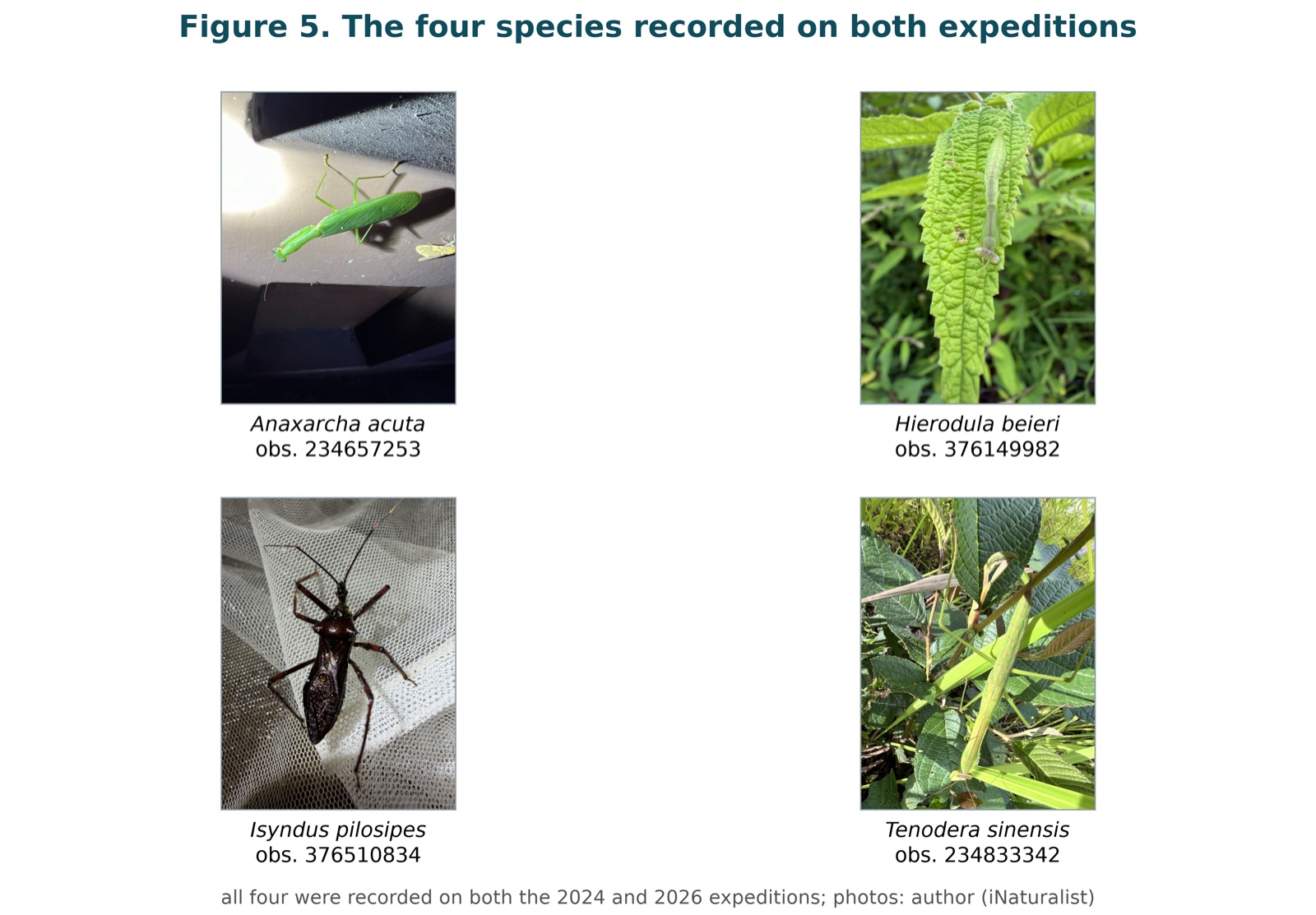
Season effect: only 4 species (all large, conspicuous predators: two mantises, a flower mantis and an assassin bug) were shared, so turnover between early and late summer appears high.
Identification effect: 27/49 (2024) and 76/118 (2026) records are not yet resolved to species, so the number of “unique” taxa is probably inflated for 2026.
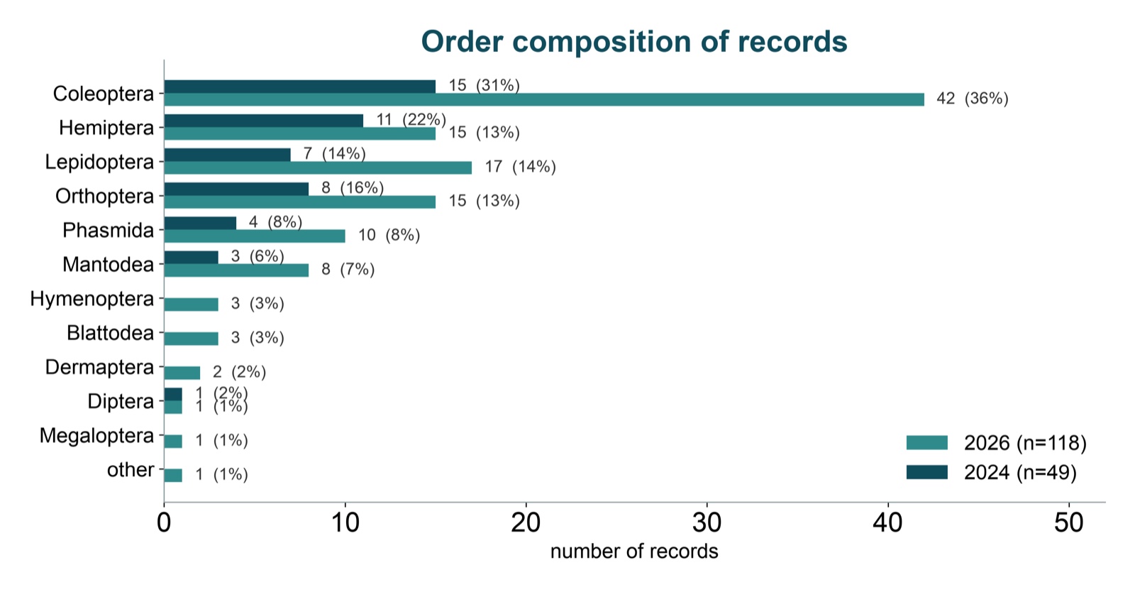
Both trips relied on light trapping, which over-represents nocturnal, phototactic groups (beetles, moths) and under-represents day-active taxa (butterflies, many Orthoptera). A UV-A source (365–395 nm) strengthens this skew (Kamei et al., 2021; Longcore et al., 2015; Schofield et al., 2023).

Conclusion

In Medog County the two expeditions differed 2.4-fold in records but only marginally in per-day discovery rate (5.5 vs 5.9 species/day). Species composition, however, was largely season-specific: only 4 of 59 species-level taxa were shared. Short, method-consistent surveys can be compared per unit effort, but detecting real change needs standardised, repeated sampling across seasons.

References

Barbato, D. et al. 2021. Light and shade of citizen science for less charismatic invertebrate groups: quality assessment of iNaturalist nonmarine mollusc observations. Journal of Molluscan Studies 87(4): eyab033. doi:10.1093/mollus/eyab033
Busse, A. et al. 2022. Light and Malaise traps tell different stories about the spatial variations in arthropod biomass and method-specific arthropod abundances. Insect Conservation and Diversity 15(6): 655–665. doi:10.1111/icad.12592
Gotelli, N.J. & Colwell, R.K. 2001. Quantifying biodiversity: procedures and pitfalls in the measurement and comparison of species richness. Ecology Letters 4(4): 379–391. doi:10.1046/j.1461-0248.2001.00230.x
Hirao, T. et al. 2008. Effects of mobility on daily attraction to light traps: comparison between lepidopteran and coleopteran communities. Insect Conservation and Diversity 1(1): 32–39. doi:10.1111/j.1752-4598.2007.00004.x
Hochmair, H.H. et al. 2020. Evaluating the data quality of iNaturalist termite records. PLOS ONE 15(5): e0226534. doi:10.1371/journal.pone.0226534
Kamei, M. et al. 2021. Effects of replacing outdoor lighting with white LEDs with different correlated color temperatures on the attraction of nocturnal insects. Applied Entomology and Zoology 56: 225–233. doi:10.1007/s13355-021-00729-7
Kishimoto-Yamada, K. & Itioka, T. 2015. How much have we learned about seasonality in tropical insect abundance since Wolda (1988)? Entomological Science 18(4): 407–419. doi:10.1111/ens.12134
Li, C. et al. 2015. White-cheeked macaque (Macaca leucogenys): a new macaque species from Medog, southeastern Tibet. American Journal of Primatology 77(7): 753–766. doi:10.1002/ajp.22394
Li, X. et al. 2020. Camera-trap surveys reveal high diversity of mammals and pheasants in Medog, Tibet. Oryx 55(2): 177–180. doi:10.1017/S0030605319001467
Longcore, T. et al. 2015. Tuning the white light spectrum of light emitting diode lamps to reduce attraction of nocturnal arthropods. Philosophical Transactions of the Royal Society B 370: 20140125. doi:10.1098/rstb.2014.0125
Myers, N. et al. 2000. Biodiversity hotspots for conservation priorities. Nature 403: 853–858. doi:10.1038/35002501
Schofield, J. et al. 2023. The colour temperature and placement of LED lighting near rivers can reduce attraction of flying adult caddisflies. Freshwater Biology 68: 2095–2108. doi:10.1111/fwb.14177

Data and figures

iNaturalist observations by the author (account xuanye), Medog County, Xizang, China. Base map from Mapzen / AWS Open Data terrain tiles, with elevation from NASA SRTM (2013). Figures produced by the author with Matplotlib, NumPy, matplotlib-venn and Pillow. All points in Figure 1 are the author’s own GPS records.